|
A Guide to Implementing the Theory of
Constraints (TOC) |
|||||
|
Replenishment – Adding Value Through The
Supply Chain Replenishment is the method by which we add
substantial value to the supply chain.
We achieve this by increasing the throughput generated from the final customer
– our constraint. In fact we must
subordinate our whole supply chain to the constraint. That is we make sure that we have exactly
the right stock, in the right place, whenever someone wants to buy it. Sound difficult? It’s not really. Not, if we think about what we are setting
out to achieve. Let’s step back for a moment to the manufacturing
cases that we have examined and the step forward into supply chain. Previously, in section on production, we
discussed increasing the throughput in make-to-order environments, an
environment where timeliness is an explicit concern. We then examined make-to-stock and
make-to-replenish environments, places where timeliness is less obvious but
still a critical element. We
represented our make-to-stock environment something like this;
Of course not all businesses contain a production or
manufacturing process, that is, there may not be any transformation of goods
carried out in the process. Instead,
value is added by moving goods through both space (transportation) and time
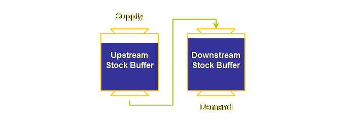
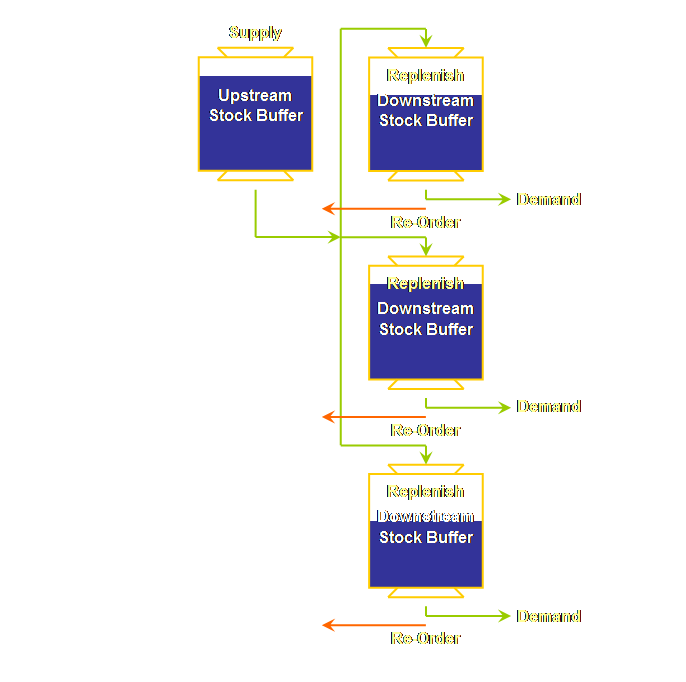
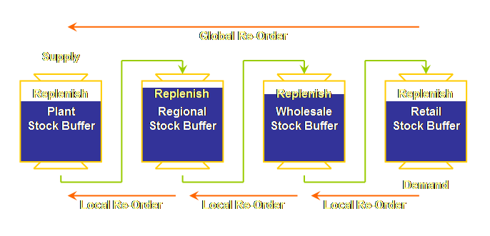
(storage) from a source of supply to the location of a demand. Rather than a flow from a process to a
stock buffer as in manufacturing, we now have a flow from stock buffer to
stock buffer. Let’s draw this.
Each node could represent the quantity of a single
type of stock unit in the chain as it passes from distributor to wholesaler
to retailer for instance. Equally we
could consider it to be the whole sum of all the different types of stock
units at each of these stages. The
diagram is generic; we can decide as the situation demands. Clearly we could also have hybrid systems with both
manufacturing and supply chain components, and the supply chain component
might not be linear; but let’s leave these interesting facets until the
distribution and marshalling pages. Replenishment is the motor for supply chain, it is the
mechanism that ensures that we never miss a sale by not having the right
material in the right place at the right time for the customer. Let’s have a closer look at the drivers of
replenishment, but first, if you have a manufacturing background you might
consider a small diversion. Replenishment can be broadly described, or defined, as
the frequent and rapid replacement of recent actual demand. The key is that there is no forecasting
into the future, only the rapid response to the very recent past. We address timeliness in supply chain by
the replenishment characteristics of our stock buffers. Through replenishment we can supply more
goods in total, to the right place, at the right time, and most often with
considerably less total stock in the system.
The objective of course is to increase Throughput. Each and every stock type at each and every node
becomes its own replenishment buffer.
The size and serviceability
of the stock buffers is driven by how frequently and how rapidly we
choose to replenish consumed stock and
this is how we configure the solution.
The configuration will depend upon the assumptions that we are willing
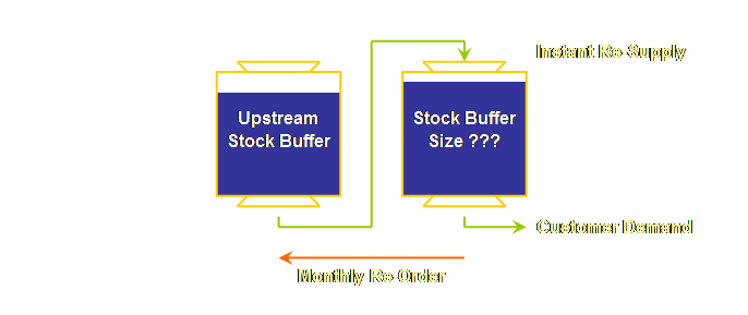
to challenge about batching; both batching in time and batching of quantity. Let’s draw this as a simple model.
Locally, the buffers, once in operation, signal
replenishment quantities – our local prioritization system – they also absorb
many small variations as well as providing day-to-day exception reporting indicating
that there may be a potential stock supply violation – our local control. Let’s add these local features to our model.
Let’s now examine a little more about what we mean
by replenishment. Replenishment is one of those words, like for instance;
quality or strategy, which means different things to different people
depending upon their work environment and their experience. This is sufficient to cause quite a bit of
confusion. In fact, it is probably
fair to say that manufacturers have one view of replenishment and that supply
chains have another view. In general it seems that replenishment
of a stock buffer is composed of two critical components; Re-Ordering and Re-Supply However, I will argue that there are at least 4
components and that the two additional ones should be insignificant, or at
least rendered so. Nevertheless we
should recognize their existence; Re-Checking, Re-Ordering, Re-Supply, and
Re-Stocking Clearly, then, re-ordering and re-supply are the two
aspects that may require the longest durations and hence impinge most upon
our timeliness and the determination of the size of our buffers. We need to examine re-ordering and re-supply
separately before combining them together once again. In order to do this let’s exclude re-supply
for the moment by something similar to that which applied mathematician do;
“let us assume” re-supply is near instantaneous! If we do this then we can isolate some of
the assumptions about re-ordering. Let’s consider 2 re-ordering environments. 1. Fixed re-order quantity variable
re-order frequency – batch lot manufacturing 2. Variable re-order quantity fixed re-order frequency – shipment lot supply chain In fact there is a 3rd which we touched upon in
manufacturing make-to-stock on the drum-buffer-rope page and which we will
mention once again after considering the mechanism for determining buffer
status. However, of the two above, the
first, fixed-quantity, is very common in manufacturing, the world of batch
lots. The second is fixed-frequency
and is very common in supply chain, the world of shipment lots – and the
subject of this page. Clearly there is tremendous potential for people to
say “I understand what you mean by replenishment,” when indeed the
understanding is locked into the first case.
I know, “I’ve been there, done that.” So let’s work through both of these cases under the
assumption of near-instant re-supply.
Then we will have a look at the effect of non-instant re-supply, and
how to accommodate this as part of replenishment. If we think about it, all make-to-stock is
replenishment of sorts. If we make
4000 new things that are standard items, and they don’t age, then it really
doesn’t matter if we make a year’s supply and put them in the warehouse –
although it would be better to be privately owned to embark on such a mission
these days. Our only risk is that the
demand might be for more than this plus our safety stock before we get around
to producing these things again; therefore we might miss sales. If we sell less than 4000 in a year, then
we just won’t make the remainder next year and bring our stock back up –
right? So in effect we did replenish the stock, it’s just
that the cycle time is quite long.
This is OK for companies with really deep pockets and really mundane
things – industrial things. I’m not
sure if we could find such a company still doing this today, well at least
not on major items, but there certainly are stable established industrial
firms who manufacture small volume items in their range once or twice a
year. However, hopefully we are all in
the business of making things to sell rather than making things to store. What would happen then if we are supplying consumer
goods or are making perishable items?
Now if we make 4000 things it’s just quite possible that the market
taste may change, or our competitors may bring out something ”new and
improved” – even if it is only the label, or that some of the stock will pass
it’s “use-by” date before it is sold.
Now we risk not only missing sales if sales are greater than our
forecast, we also have a very real risk of dead stock. So what would happen if instead of making 4000
things once a year we made 1000 things once a quarter or heaven-forbid 333
things every month, or 83 and bit every week?
Oops, round that up to 84 for safety – no make it 85. Can you see where we are heading? We are always replenishing whether with
4000 things or 85 things, but with increasingly smaller quantities and
increasingly higher frequency.
Moreover, because we are externally constrained and have processing
capacity to spare, we can chase any localized market spurts, and we can also
drop off quickly with any market downturns.
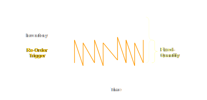
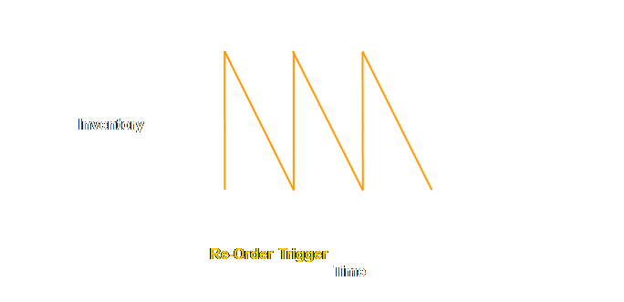
In a word we have become responsive. Let’s examine this graphically. Let’s retrieve our diagram for a
hypothetical stock item from the finished goods section. A perfect saw-tooth diagram.
We know from discussions of batch sizing throughout
this site that reducing the process batch size will reduce the amount of
inventory required to be held in finished goods and that there will be a
equivalent increase in replacement frequency.
Let’s draw this.
Effectively as batch size decreases the maximum
stock in absolute terms approaches closer and closer to the re-order point
stock level. Of course the ideal batch
size would be a unit of 1 – single piece transfer/just-in-time. Therefore replacement in a processing environment is
characterized by; Fixed
Re-Order Quantity & Variable Re-Order Frequency The process requires a finished goods stock – but it
should be as small as possible to decouple the customer from the
process. The customer can still get
stock immediately, and the process replaces it with as small a batch as
possible. In re-order point systems the batching policy is
explicit. However, in some min-max
systems the batching policy may be more implicit; “the batching policy is
hidden under the size of the max minus the min (1).” The batch size is defined by the physical
and especially the policy constraints of the process. Most manufacturers will recognize the above
discussion as what they term replenishment – and this type of fixed-batch
replenishment does find its way into supply chain too. However, it generates two traps that we
should be aware of and try to avoid. The first trap comes from synchronization. Consider the following.
How could such a synchronization arise in the first
place, from simple chance? Or did it
arise from the last synchronous re-supply from the upstream node? This seems far more probable. Often times we create our own problems for
ourselves. This type of problem
creates large waves in upstream nodes when gentle and continuous downstream
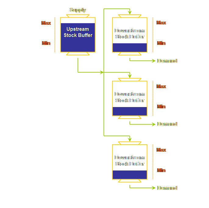
consumption is the reality. The second trap comes from the number of layers or
levels of nodes in the supply chain.
Combine these two situations, a significant number
of layers and some one-to-many relationships and then even a simple linear
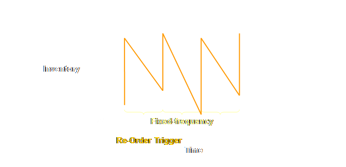
supply chain is suddenly not so simple any longer. Let’s look at the alternative then; fixed re-order
frequency with near-instant re-supply; a more common replenishment system
found in supply chains. In supply chain, as opposed to manufacturing, it is
possible to break out of fix-quantity re-orders and instead fix the re-supply
frequency. So we need to investigate
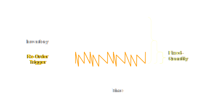
this as well. Let’s start again at the beginning once again with
our perfect saw-tooth graph.
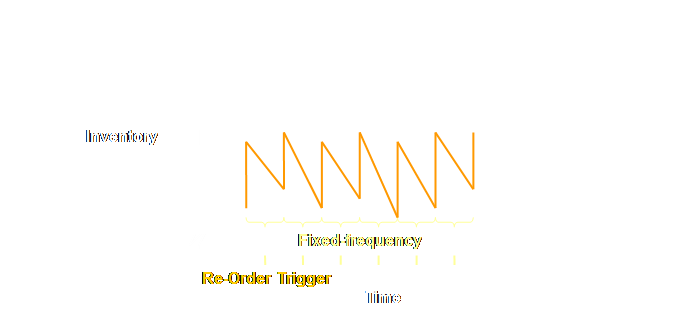
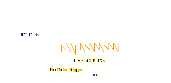
Just as in the processing environment where we could
reduce the quantity in each batch, here we can increase the frequency and
obtain the same effect; reduced inventory of finished goods stock without
degrading service levels. Let’s halve
the re-order date duration and thereby double the re-order frequency. This is the equivalent of ordered once a
fortnight instead of once a month, or ordering once a week instead of once a
fortnight.
Therefore replenishment in supply chain environments
is characterized by; Variable Re-Order Quantity & Fixed Re-Order Frequency Many times the variable quantity that we re-order to
in fixed-frequency re-ordering is in actuality a forecast value for future
expected consumption. Many of the ERP
systems that generate these targets are operated on a monthly cycle ensuring
large quantities that are produced infrequently. The two traps that we mentioned for min/max systems
still operate to some extent. In terms
of the one-to-many relationship and synchronization, if all the nodes
re-order on the same date, this will cause a “”wave” of demand on the
upstream supply nodes when the customer drawdown might have been quite gentle
and uniform during the preceding period.
In terms of the number of layers of levels of nodes, it can still take
a loooonng
time for a signal from the customer node to arrive back at the source node . Depending
upon the order dates it could take as many replenishment cycles as there are
nodes for a point of sale signal to arrive back at the first node. None of this will surprise anyone in supply
chain. But what can we do about it? We know how to significantly reduce the size of a
stock buffer by either smaller quantities or more frequent re-supply. Classically we achieve one by fixing the
other. Hopefully this analysis has
allowed manufacturers to break the fixed batch quantity mind-set that is
sometimes carried over into supply chain.
In supply chain we fix the frequency and this is the path that we will
follow here in our development of replenishment buffers. Let’s have look, then, at this thing called a
replenishment buffer. Let’s examine buffers in a different fashion to the
saw tooth diagrams that we have used to date.
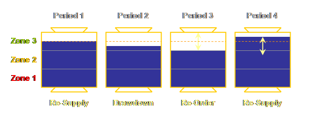
Let’s draw some fixed-frequency replenishment buffers over a complete
cycle and see if that further helps to draw the distinction between the two
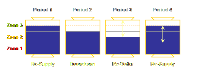
environments of operation – processing and supply chain. Let’s first look at normal
demand.
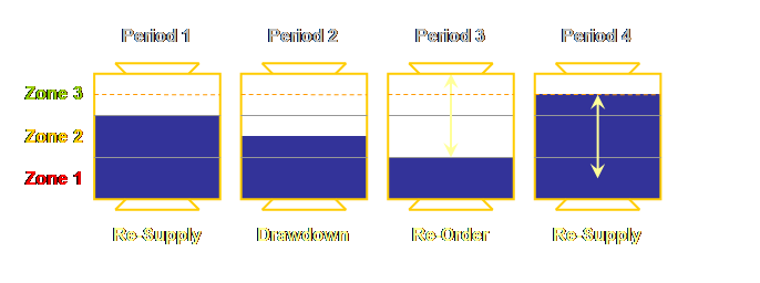
Let’s have a look at this system if we started with
a relatively less stock in the buffer
to being with but at the same rate of drawdown.
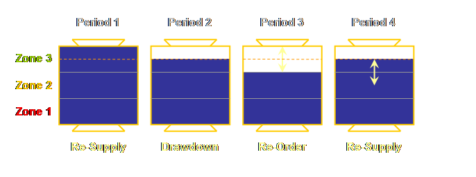
What then if we were to start with a relatively more stock in the buffer to begin with but at
the same rate of drawdown? Let’s look
at that.
In this particular example there appears to be some
robustness about the buffer design with respect to the rate of stock
drawdown. Therefore let’s look at both
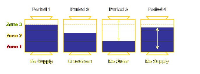
a substantially greater and substantially reduced rate of drawdown. What happens then during a period of heavy
drawdown? Let’s use our original case
but we will increase the rate of drawdown by 50%. Let’s have a look at that.
Let’s then have a look at periods of light
demand. Again we will use the initial
case but we will decrease the demand by
50%.
On the drum-buffer-rope page I tried to make a
conceptual distinction between fix-frequency buffers of make-to-replenish and
the classical fix-quantity buffers of re-order point and min/max of
make-to-stock. I suggested that
fixed-quantity min/max buffers might be viewed as filling from the bottom and
that fix-frequency replenishment buffers – like we have just drawn above –
might be view as filling from the top.
If we fill from the top, then we need to know just how big the buffer
is. We need to know how to size the
buffer. Let’s pool our knowledge of
decreasing batch size and increasing shipment lot frequency and address how
to size a supply chain replenishment buffer. A supply chain replenishment buffer must protect the
downstream node, or the customer demand if it is the last node, from
fluctuations in both downstream demand and in upstream supply during the
period of interest. The period of
interest is the replenishment time.
The replenishment time we already know is composed of the re-order duration and the re-supply
duration. However, so far we have fairly much assumed
near-instantaneous re-supply. Let’s
continue to do that for a while because I think that it will help us to
understand better the various components of replenishment. Let’s start with a simple case – two nodes.
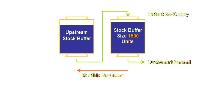
Buffer Size = Average Recent Demand In The
Re-Order Period An initial suggestion for a good value of safety is
plus 50% (3). Such a suggestion
automatically creates a buffer zonation of 2/3rds to 1/3rd (more on that
later). A more recent verbalization for the buffer size is;
the maximum forecasted consumption within the average replenishment time,
factored by the level of unreliability of re-supply (4). It seems that the term “re-supply” was however
used loosely to mean all of the replenishment duration rather than a specific
component of replenishment duration as we are using it here. This was corrected in the Insights program
on distribution and supply chain as; the maximum forecasted consumption
within the average replenishment time, factored by the level of unreliability
of replenishment (5).” Thus the more variable the customer demand, the
bigger the buffer. The more variable
the re-order duration, the bigger the buffer.
The more variable the re-supply duration, the bigger the buffer. The higher the required customer service
level, the bigger the buffer. These
situations are better accommodated in the later verbalizations. With this in mind, however, let’s stick
with the first formula; it will help us to better understand the situation if
we limit ourselves to this more straightforward case. Let’s assume some numbers. Let’s assume that we sell 1,000 units per
month on average. With near-instant
re-supply our buffer size is 1,500 units.
Lets draw that.
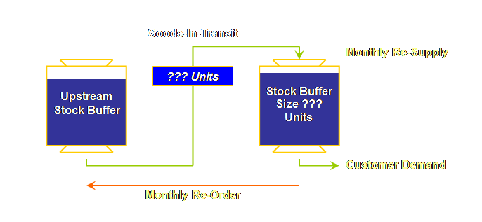
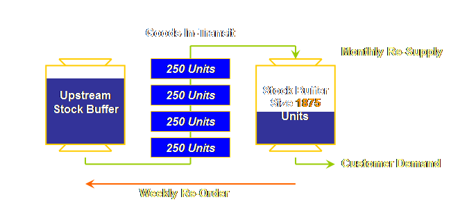
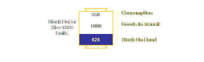
What if we can’t get re-supply next day from across
town? Well, then we have to make the
buffers bigger. Let’s have a look at
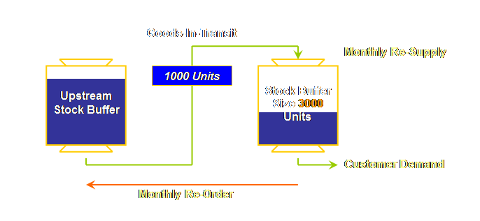
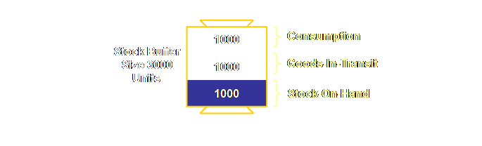
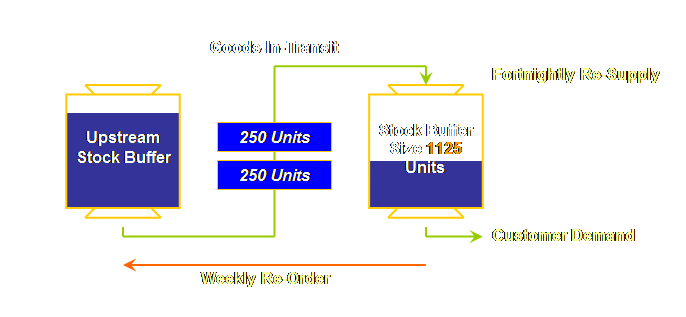
that. What if we order monthly but the shipment comes
across country or across the sea? We
have to take that into account too.
Let’s start with monthly re-ordering and a month to re-supply.
But let’s not forget, the objective is not inventory
reduction per se, it is getting the right stuff
to the right place at the right time so that our throughput goes up, so that
our customers come back to us for more (and not our competitors), and so that
our throughput goes up even further. It seems any time someone makes a suggestion for
smaller batches and more frequent delivery, someone else will raise the issue
that operating costs will go up. There
is a very good discussion by Cole on why operating costs should, in fact, go
down while addressing this particular aspect and a myriad of other aspects as
well (2, 3). However, please also
check out the “truck and trailer” analogy in the production page on batch
issues. There are graphs there that are
relevant to supply chain. From these
we can infer that it is very likely that a significant proportion of the
active inventory in any supply chain is in actuality the smaller part of the
total shipment lots. More frequent
re-supply of this portion of the stock will have considerable leverage upon
the whole system without substantially increasing the total shipment lots. Once we have determined the buffer size, how do we
determine the replenishment amount? The only pieces of information that we have are the
buffer quantity that we are aiming for, the quantity present as stock-on-hand
at the re-order date, and any goods-in-transit. Thus the replenishment amount is the
difference, and as depletion will continue to occur until replenishment is
achieved, then the replenishment when it does arrive will be to a less than
the full buffer. Re-Order Quantity = Buffer Quantity –
Stock-On-Hand – Goods-In-Transit + Orders The re-order quantity is fairly much the same as the
proportion that we have been calling consumption above. In fact it should be fairly clear that the re-order quantity replenishes consumption. Of course it would be easier to write “re-order
quantity = consumption” but the amount of consumption only has relevance with
respect to the buffer quantity that we establish. So it has to be determined by difference. But where did that “orders” term suddenly come
from? Well, “that would be the
computer!” You see often times the
order processing people put an order against a stock unit which remains
currently unpicked but nevertheless committed to a customer. The most obvious cause is waiting for
transportation. We could leave the
term out, but seeing that we have made a firm commitment to sell it in the
near future we may as well replace it sooner rather than later.
If your experience is confined to supply chain, it
may seem unusual to even consider why the replenishment buffer should be
determined by anything other than quantity.
However, on the drum-buffer-rope page, we labored the point that in a
manufacturing process the size and activity of the constraint, control point,
assembly, and shipping buffers are measured in units of time. This is a unique feature (#). It is a consequence of the acknowledgement
of the existence of a singular constraint within a process. For constraint buffer activity we said
that; At a manufacturing constraint an hour is
an hour but the number of units may differ. The number of units differs due to the fact that different
types of product using the same constraint may use different amounts of
constraint time. The unique
perspective brought about by the recognition of a singular constraint allows
us to define the length of the buffer in time also. Essentially the buffer is sized and “sees”
the duration from the gating operation to the constraint due date. Moreover the buffer “sees” committed demand
– work that has been released to the system. Why then, doesn’t this carry over into supply chain
replenishment if it is so important in drum-buffer-rope manufacturing? Well, in a way, it does as we shall
see. Replenishment buffer size and
activity is defined by time but is measured by quantity. Why is this? Let’s examine replenishment buffer activity first. The clue comes from the buffer sizing discussion
earlier when we used the “average recent demand.” Even when the re-order and re-supply
periods have military regularity to them, the actual amount will vary because
the demand rate varies over time.
Therefore, the amount of time or demand that our material stock can
“cover” is variable. Sometimes demand
is high and we utilize units faster and over a shorter period. Sometimes demand in low and we utilize
units slower and over a longer period.
But a unit is still a unit.
Thus; At a replenishment node a unit is a unit
but the hours may differ. In replenishment where nothing is undergoing
conversion or combination – there is no processing – then we use units of
quantity to measure buffer activity. What about the replenishment buffer size then? The unique perspective brought about by the
designation of a replenishment node allows us to define the length of the
replenishment buffer in time.
Essentially the buffer is sized and “sees” a duration that extends through
one period of the re-order and re-supply cycle. However, the buffer now “sees” uncommitted
demand – we can not tell how much we will sell in the next hour or day or
whatever. Therefore, we must once
again substitute “non-variable” units of stock in place of the “variable”
amount of time or demand that they “cover.”
Thus the replenishment buffer size is also measured in units of
quantity. Both manufacturing and supply chain buffers are defined
by time; the period that the buffer “sees.”
However, in supply chain we measure buffer size and activity in
units of material, and not in units of time. We called replenishment the motor for supply chain
solutions. Re-order and re-supply
duration determine the buffer size and are the characteristics which
configure the system. Buffer
management is the monitoring and control function that we use once the
configuration is in place. Schragenheim describes the role of buffers and
buffer management in replenishment as follows. ”Instead of trying to be very precise in
very uncertain situations (like using sophisticated forecasting techniques),
TOC strives to build a robust design that is good enough. The initial parameters are based on crude
forecasting that is complemented by crude assessment of the variability of
both market demand and replenishment time.
What complements good-enough planning is a very flexible and
priority-driven execution control system that is capable of taking care of
the exceptions.” “Buffer management is
a control mechanism. The idea behind
it can be summarized as: identifying situations where the planned protection
is almost exhausted (1).” Buffer management is a benign form of control,
basically, it is reporting by exception.
Thus we focus on the few things that are locally important and we
don’t focus on many things that are locally unimportant. There are two mechanisms by which we can manage our
buffers. The first and older method is
buffer zonation, Schragenheim and Dettmer call this “traditional buffer
management (6).” The second and more
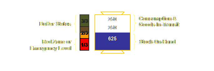
recent approach is buffer status (1).
Schragenheim and Dettmer described the precursor to buffer status (in a
manufacturing make-to-stock environment) as the “S-DBR approach” to
controlling uncertainty and variation (7).”
Let’s work through the buffer zonation approach first, leading onto a
discussion on local performance measurements, and then we can examine the
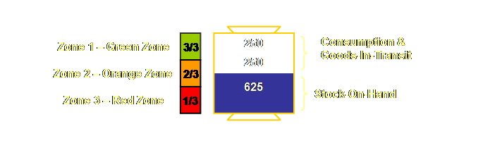
more recent buffer status approach. In fact we have mentioned buffer zones in passing
throughout this page. As with the
manufacturing logistical solution (or project management for that matter),
the buffer is divided into three. These are referred to – from nearly full to
nearly empty – as; zone 3 (the green zone), zone 2 (the orange zone) and zone
1 (the red zone). It refers only to
the stock-on-hand, the stock that we have that we can use to immediately
fulfill a new order. Let’s show this.
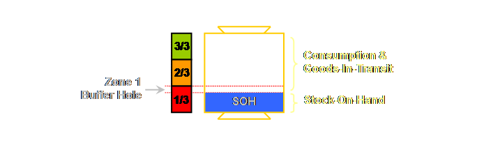
A zone 1 stock buffer penetration offers us two sets
of information. The first is a simple
record of an incidence – we have a hole.
The second piece of information is the magnitude of
the depletion. Now things become more
interesting. Unlike a make-to-order
manufacturing environment, where each job is discrete with an absolute
delivery date, and the magnitude of a buffer hole can be quantified when the
job is finally completed, make-to-stock is continuous – we continuously
replenish and customers continuously deplete our replenishment. So, we can not put a mark in the ground
that says “hole closed on this day.”
Instead we must continuously monitor the number of units missing from
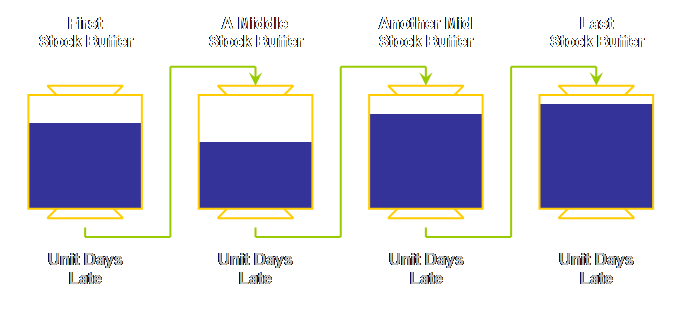
zone 1 and the number of days that they are missing for. We must record the number of units “missing” from
zone 1 each day that any units are missing and we must aggregate this over
our reporting period – be that a day, a week, or a month. The measure is unit-days late. Note that it is an absolute measure based
upon the quantity of material and the amount of time. Now we must put a value to this
measure. Let’s look at local
performance measures. There are two local performance measures. They are measures of local unit-days-late,
which we have just examined, and local unit-days-wait. We can attach values to these in for-profit
systems and call them throughput-dollar-days late and inventory-dollar-days
wait. We know the fundamental or system-wide measures for
a for-profit system; they are throughput (sales minus totally variable costs
excluding direct labor), operating expense (including direct labor), and
inventory (all capital investment).
However we can’t and don’t want to apply these to sub-systems or else
we are going backwards to a reductionist/local optima approach. In a supply chain however, it may be that
each subsystem is indeed a separate business with its own throughput,
inventory, and operating expense.
Nevertheless we can still use the two local performance measures to
ensure alignment of the whole supply chain. If we can’t supply an order ex-stock at the time
requested then that order is considered to be late. We operate the system to take account of
dependencies and variation so we would hope that nothing is late. The measure of lateness is the value of the
goods (throughput) multiplied by the number of days late to obtain throughput-dollar-days. It seems that we can apply this measure to
two different places. We can apply
throughput-dollar-days lateness value to zone 1 buffer penetration for internal
measurements (8) and order non-fulfillment for external measures (4). For the external measure we should aim for
a zero value. Thus, whenever there is
a hand-off within the supply chain we can expect to use a value of
unit-days-late. Let’s draw this situation for a simple supply chain.
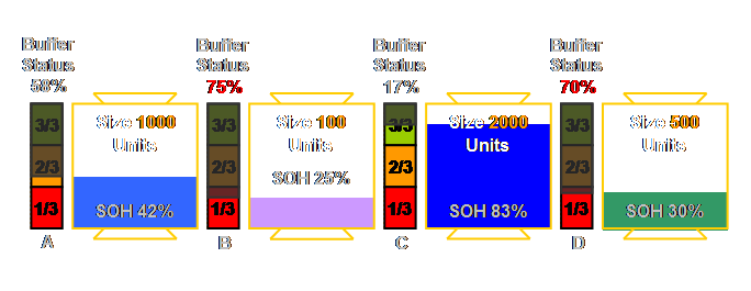
Schragenheim uses the term “buffer status” to refer
to buffer consumption or buffer penetration (1); where buffer status is: Buffer Status = (Buffer Quantity –
Stock-On-Hand) / Buffer Quantity In this situation the buffer status value is the
inverse of the proportion of stock-on-hand.
Let’s draw this.
Consider the buffer status of 75% for stock item B
above. In absolute terms this
represents an incursion of (0.75-0.66) by 100 = 9 units. Consider the buffer status of 70% for stock item D
above. In absolute terms this
represents an incursion of (0.70-0.66) by 500 = 20 units. We might be tempted to pay more attention to the
goods-in-transit for stock D than the goods-in-transit for stock B, but stock
B is more important, the buffer status is worse. Cole considers that there are 3 reasons that might
lead to a resizing of a buffer once it has been set (2). They are; (1) Buffer is too small (2) Buffer is too large (3) Seasonality or promotions Using Schragenheim’s criteria, a buffer is too small
if penetration into zone 1 is too frequent and too large if penetration into
zone 1 is too rare (1). Using average values of consumption and re-order and
re-supply as we have here, it might be assumed that half the time our zone 1
would be too small and half the time it would be too large. In fact this is correct, but the period
over which it concerns us is near the end of each re-order period. So, for instance, if we have a monthly
re-order period we may penetrate into the red zone – near the end of the
period. But how long do we do this
for? If it is one or two days out of
20, then we have a zone 1 penetration of 5-10% of the total time – not 50% of
the time as we might first expect. Let’s look then at seasonality. There is a demand for electric fence energizers for
pastoral farming. The electric fences
– often a single wire set a little below a person’s hip height – keep cattle
in the pasture eating what they should eat and out of the areas that they
shouldn’t eat. And although cattle can
stretch their necks a surprisingly long way, on the whole this is a very
effective system. Dogs who insist on
holding their tails upright while passing under these fences will also attest
to their efficacy. However, grass grows at the greatest rate in spring,
and this is often when electric fences are used to “break-feed” new
pasture. Thus the majority of the
demand for electric fence energizers occurs within 2-3 months. How do we ensure that we sell all the
energizers in all the model configurations that are desired in the quantities
required without either leaving some demand unsatisfied (because then the
sale may fall to a competitor) and without leaving excess and unsold stock to
carry for at least the next 9-10 months? We need to set a seasonal buffer for this
example. Firstly why don’t we estimate
the maximum expected sales that we could hope to make by the end of the peak
sales period. Secondly we need to
determine the available production capacity during the peak period. We then subtract the amount that can be
produced during the peak sales period from the maximum sales amount and this
becomes our pre-peak target buffer. We
build to this buffer prior to the season and then once the season is underway
we can chase the peak with our existing capacity. We can therefore be assured that we won’t
get left with too much excess stock to carry and we are also assured of
meeting our most favorable estimate for sales. We examined this topic on the drum-buffer-rope page
in the production section, but let’s revisit it here. Supply chains can occur “free standing” as
we have examined then here, or they can occur in combination with
manufacturing either after or before a manufacturing process. Now that we have a much better
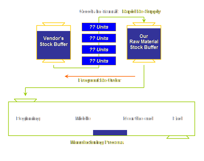
understanding of how to utilize replenishment buffers lets re-check this
understanding against raw material or inwards goods stock buffers. Let’s draw a basic diagram of the
situation.
Vendors, unfortunately, are one of those groups were
it is very easy to externalize the challenges of managing the system and
blame the vendors. Well, we can do that.
However, ask yourself, will it cause anything to improve? We might even be able to change vendors –
until the next vendor goes “bad” on us too.
Vendors really are beyond our span of control and most often our
sphere of influence as well, so about the very best thing we can do is to
buffer ourselves against their impact upon our business. We can modify our basic replenishment formula
to account for vendor behavior. Here
it is. Buffer Size = Maximum Expected Demand In The
Longest Re-Order Period Such a more conservative buffer sizing; “maximum
expected demand” and “longest re-supply period,” may cause some inventory
levels to go up, but we have to ask ourselves whether we are in the business
of making money through sales or in the business of saving money through
reduced inwards goods. If we are still
not happy, then we should try and persuade our vendor to own the goods until
we consume them. That way the vendor
will learn something about the cost of their own (un)reliability. Better still, we should try to reduce the
inventory size (if necessary) by increasing the frequency of the re-order and
decreasing the duration of the re-supply while fully protecting our own
throughput. How can we compare what we have learnt here with
traditional supply chain management?
Maybe it is best to think of current supply chain management as the
reductionist/local optima solution for distribution, just as MRPII is the
reductionist/local optima solution for processing or critical path is for
project management. Traditional supply
chain management uses forecasting to try and overcome the long lead
times. The long lead times generate
large work-in-process but somehow as a consequence we never have all the
right things in the right place at the right time. Instead we have challenged the very need
for such long lead times. No matter
how good or how expensive our software solution is, if it is using
traditional reductionist philosophy; we won’t be able to put the right
protection the right place to drive system profitability. The only way to overcome that is to use
replenishment buffering, we can best evaluate the impact by examining the two
traps that we discussed earlier. The
first was synchronization caused by a one-to-many relationship between source
and demand.
What then, if we have several layers of nodes in our
system?
If we are willing to challenge that we must forecast
and that re-order and re-supply times must be in-frequent then there is much
we can do to ensure that the supply chain functions with precision and
profit. We have looked at 2 replenishment environments; 1. Fixed re-order quantity variable
re-order frequency – batch lot manufacturing 2. Variable re-order quantity fixed re-order frequency – shipment lot supply chain But there is a third 3. Variable re-order quantity and variable re-order frequency We touched upon this in the drum-buffer-rope page in
the section on manufacturing make-to-stock and discussed the rules required
to action it. Within a manufacturing
system it is possible to launch new stock orders at any time based upon a new
stock order release priority determined by the relative stock order status
for each stock buffer. Schragenheim
showed how this becomes a self-regulating system (1). There exists a potential to extend this
mechanism into supply chain; especially those that are computerised. Consider once again that replenishment is composed
of the following; Re-Checking, Re-ordering, Re-Supply, & Re-Stocking It stands therefore that whenever re-checking is
more frequent than re-ordering, and re-ordering is already frequent, that
there may be re-checking periods when there is no re-order quantity required,
or the re-order quantity for a re-order period is smaller than one that we
wish to commit to. In this case our
re-order frequency has become variable rather than fixed. The more frequently that we are able to
re-check and re-order the more likely that our re-order at any one time for
any one stock may be less than we wish to commit to. Thus we have variable re-order quantity as before,
but we now also have variable re-order frequency as well. This appears to me to be a natural
progression as shipment lots become more frequent and smaller. It is an ideal which we should aim to work
towards.
We can summarize this as a simple table.
Using correct buffer sizing criteria we can ensure that
we can always supply the next node in our supply chain to the desired level
of service regardless of the variability or reliability of our vendors or of our
customer’s demand. Moreover, reduction of the re-order duration and
reduction of the re-supply duration can reduce the overall inventory in the
system substantially while increasing overall service levels. Nevertheless, the objective is not
inventory reduction per se it is
increased throughput. Next let’s see how we can apply this to two particular
configurations, divergent supply chains in distribution, and convergent
supply chains in marshalling. (1) Schragenheim,
E., (2002) Make-to-stock under drum-buffer-rope and buffer management
methodology. APICS International
Conference Proceedings, Session
I-09, 5 pp. (2) Cole, H., (1998) Implementing distribution –
layers 4-5. Video JMT-16, Goldratt
Institute. (3) Cole, H., (1998) Distribution – layers 1-3. Video JMT-6, Goldratt Institute. (4) Goldratt, E. M., (2002) Theory of Constraints
self learning program of distribution and supply chain. CD-ROM, Goldratt’s Marketing Group. (5) Goldratt, E. M., and Goldratt, A., (2003)
Insights into distribution and supply chain.
Goldratt Marketing Group. (6) Schragenheim,
E., and Dettmer, H. W., (2000) Manufacturing at warp speed: optimizing supply
chain financial performance. The St.
Lucie Press, pp 123-135. (7)
Schragenheim, E., and Dettmer, H. W., (2000) Manufacturing at warp speed:
optimizing supply chain financial performance. The St. Lucie Press, pp 175-207. (8)
Schragenheim, E., (2003) Measures and trust in SCM. PowerPoint presentation link to CIRAS Center
for Industrial Research and Service - Iowa State University. This Webpage Copyright © 2003-2009 by Dr K. J.
Youngman |